How Formulas Help Excel do the Calculations for You

To see this process in action, watch the video that accompanies this post.

Microsoft Excel is a spreadsheet program that can be used to process simple computations as well as advanced functions. Most people can use Excel for basic calculations like:

• Sum - adds the numbers in the cells in a selected range
• Average - finds the average of the numbers in cells in a selected range
• Count - counts the number of cells in a selected range with numbers in them
• Countif - counts the number of cells in a selected range that meet the criteria you set

There are hundreds of formulas in Excel, but creating simple functions to start with does not take long and is fairly simple. To show how versatile some simple formulas are, consider how they can be used to track:

• Attendance and absences for a group
• Average spending or income
• Supplies for a business or event
• Inventory for insurance or a business

These are a few examples of how Excel formulas can be useful by automatically processing repetitive calculations.

How Formulas Help Excel do the Calculations for You

For this example we are creating an example spreadsheet that will add formulas to track red and white wine inventory. However, these columns could represent nearly anything you wanted to track. This example represents how items can be tracked in Excel and taking the data one step further, how formulas can make calculations automatically.

Keep in mind there are also multiple ways to orient data being tracked. Choosing whether to list the information by rows or columns is mostly preference. Either way can be effective and doing it differently than the example should not change the results.

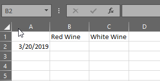
• First, create descriptive headings for the data being tracked. This will help when you access the file later, or if you share it with someone else. It is best to keep it simple when getting started and add data over time as your understanding of how a spreadsheet works increases.



• From here, enter the starting inventory under the headings created.
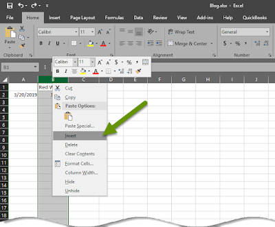
• Now, insert a column to track usage. Right-click on the letter above the column with the first heading and select "Insert" to insert a column before the current column selected.



• Add a heading to the new column created.
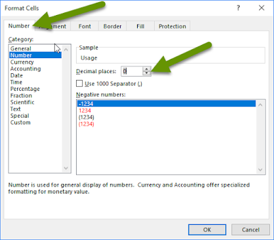
• Right-click on the letter above the new usage column and select "Format cells".
• In the Format Cells window, on the Number tab, select "Number" in the Category menu on the left and if applicable, reduce the decimal places to 0. Click "OK" to save these changes. The purpose of formatting the column data is to control how the numbers entered are processed.



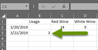
• Add additional dates to represent usage.
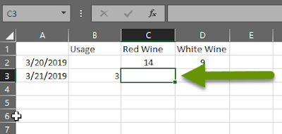
• Add a number into the usage column next to an additional date.



• Click into the cell under the original inventory amount in the first inventory column, or red wine in this example. This is where the first formula will be added.



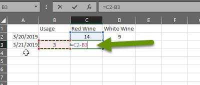
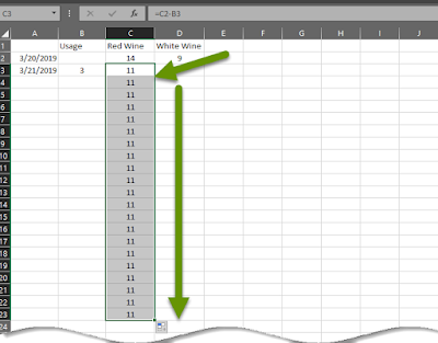
• Type a formula in this cell. In this example, we want the inventory to be represented by reducing the original amount by any usage. To do this, we will subtract any usage from the original amount and the formula would look like this: =C2-B3. This tells Excel to subtract the usage amount in B3 from the original inventory amount in C2.



• NOTE: The easiest way to enter a formula is to enter the equal (=) sign, then click the first cell included in the formula, press the mathematical expressions on the keyboard, then click on the next cell until the formula is finished.
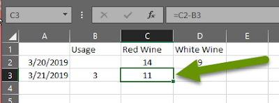
• Press the enter key and the result of the formula is automatically calculated and appears in the cell where the formula was entered.



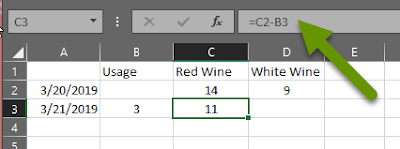
• Once a formula is entered, the resulting calculation is all that appears in the cell. However, clicking on the cell will display the formula in the box above the sheet next to the formula symbol.



• Now that a formula is entered, there is no need to enter it repeatedly down the column so that it is calculated in each cell. Instead, you copy the formula by clicking on the bottom right corner of the cell with the formula. Be sure the cursor is a black plus before clicking and dragging. Left-click and drag the cursor down the column to copy the formula. The formula will automatically update for the appropriate cells. In this example the next cell formula would be "D2-C3", etc.



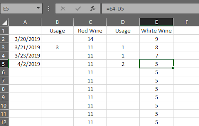
• Repeat this process to add a usage column for white wine, or whatever data you are tracking.
• Once the formula is copied down, the number in the inventory column automatically changes when numbers are added into the usage column.
• Click in any cell with the formula to verify the formula is still correct.



The formula used in the example above is fine for small situations, but does not consider adding inventory. To add inventory and have this calculated automatically, follow a similar process:

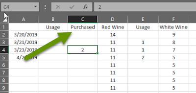
• Insert another column before the red wine inventory column and after the usage column. Name it something relative to adding inventory.



• You can add numbers into this new column, but until the formula is updated, nothing will happen with the inventory.



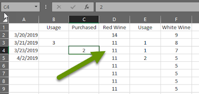
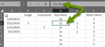
• Click in the cell with the original formula. In this case, that is now cell D3 because a column was added before it. Luckily, when rows or columns are added, Excel does its best to adapt to the changes and keep the formulas working as originally entered.



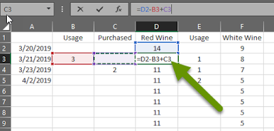
• In this example, the formula has automatically been updated to "=D2-B3" because of the added columns. Add "+C3" to the end of the formula.



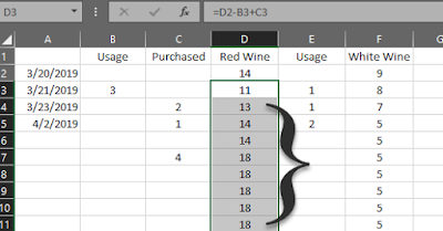
• Press enter to update the formula in the original cell. Drag the new formula down the column the way the original formula was to update the formulas in each cell.



• With the formula updated, the calculated results of the inventory column will be updated automatically based on data entered into the usage or purchased columns.
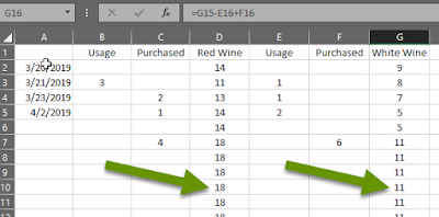
• Repeat this process for white wine so that the inventory for both items being tracked is updated automatically when used or new supplies are purchased.



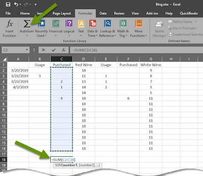
• To add a sum, say of the amount of items purchased, simply click in a cell below all the items purchased.
• Click the AutoSum function on the Formulas tab to enter a sum.
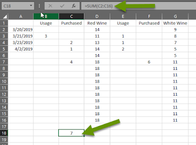
• Select the cells to include in the sum.



• Press enter and the sum is calculated in that cell.

The process for creating formulas can be as simple as adding a sum once data has been entered, or can be slightly more complicated like increasing and reducing inventory based on usage. There are also far more complicated formulas built into Excel, some of which can take a great deal of time to master. Luckily, Excel is intuitive in many ways, allowing formulas to be copied and automatically adjusting rather than requiring continual input. Additionally, when columns and rows are added, Excel accounts for this and maintains the integrity of the original formula. Overall, Excel is a powerful tool that can help anyone whether it is for personal or business usage.

As always, there are often very powerful tools available in the software we use everyday. Knowing how to get the most out of them and make them work to our advantage is how we save time and energy!