5 Lesser-Known Features that Make Excel Easier to Use

Excel is a powerful spreadsheet program that can help track, find trends, make calculations, and process entered data hundreds of different ways. Once you know how to use Excel and become more familiar with it, you will find more and more reasons for using it. Beyond the tools you regularly use, there are tons of built-in features you might not be aware of in Excel. However, knowing about these tricks makes Excel that much easier and efficient to use.

This post discusses five lesser-known features that make Excel easier to use.

5 Lesser-Known Features that Make Excel Easier to Use

The following is a list of the features you might not be aware of yet. Feel free to skip to any particular item:

1. Extending the tab bar
2. Quick accessing any tab in a workbook
3. Hiding columns or rows to only view the data you need
4. Hiding an entire sheet
5. Removing duplicate information

One of the things that can make it challenging to work in Excel is that once several tabs have been created, switching back and forth between them can feel tedious. Navigating between sheets by scrolling left and right is less than effective. Also, if you are entering functions into cells that refer to data in other sheets, creating the formulas can become time consuming.

Luckily, the bar at the bottom of the screen that shows some of the sheets in the workbook can easily be extended to fit more tabs into the viewable area.

To adjust the viewable tabs at the bottom of the window:

• Left-click and hold on the kebab menu (3-dot vertical menu) and drag it to the right as far as you want.

This allows several more sheets to always fit into the viewable area. Also, this area can be extended or collapsed at any time.

When you have a workbook with so many tabs that extending the viewable area to see additional tabs is not enough, there is another trick that allows you to quickly access any tab in the workbook.

To quickly access any tab in a workbook:

• Right-click on the arrows used to scroll left and right between the existing sheets in the workbook.This will open a pop-up that lists all the sheets in the workbook.

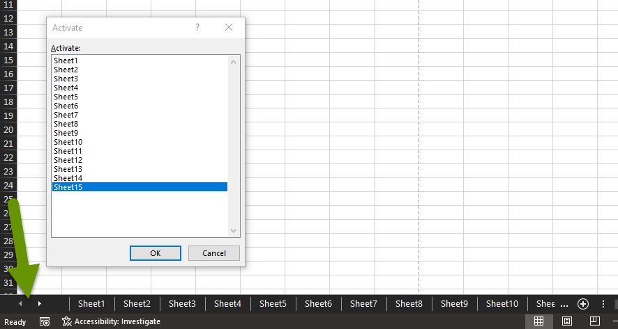
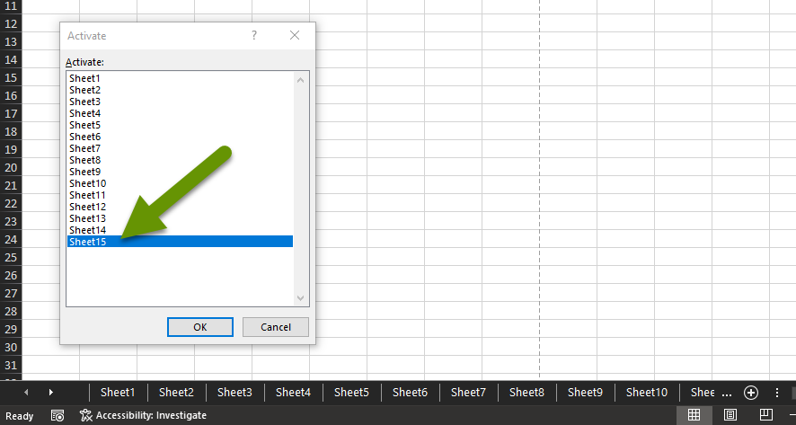
• Click on the name of any sheet and click "OK" which will take you directly to the selected sheet. This trick works from within any sheet in the workbook.

Sometimes when we create a spreadsheet and begin filling in data, we have only a limited amount of data in mind. Over time, a single sheet can end up having enough columns that they extend into double letters. When this happens, the sheet is somewhat less functional, even though you probably need all the data and breaking up the data between several sheets would be tedious.

Excel provides a way to hide specific columns without losing any of the data stored in them. This feature allows you to focus only on the data needed, hide the rest, and bring it back whenever it is needed.

To hide specific columns or rows:

• Right-click on the heading of any column or row and select "Hide".

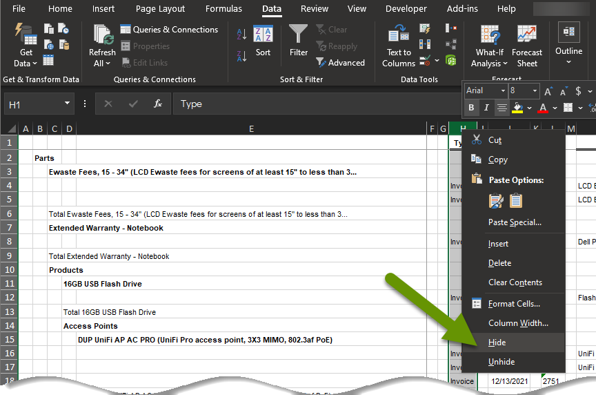
NOTE: Multiple columns and rows can be selected at the same time when hiding and unhiding columns and rows.

To unhide a column or row, highlight the columns or rows on both sides of the hidden column or row, then right-click and select "Unhide" from the pop-up.

Another thing that can make using Excel less efficient is having too many sheets. Aside from extending the viewable bar and going directly to a sheet, sometimes it is easier to hide those sheets you do not currently need and focus on only those sheets you do need. In addition to being able to hide columns and rows, Excel provides a way to hide entire sheets. One of the biggest benefits of hiding columns, rows, and sheets is that none of the data is lost and they can be unhidden at any time.

To hide an entire sheet:

• Right-click on the name of any sheet and select "Hide" from the pop-up menu.

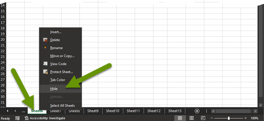
This will hide that sheet until you unhide it.

To unhide a sheet:

• Right-click on any sheet and select "Unhide" from the pop-up menu.
• This opens a window listing all of the sheets currently hidden.

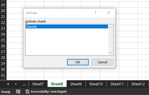
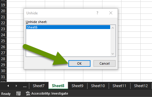
• Click on the name of the desired sheet to unhide and click the "OK" button.

Last but not least, Excel provides the ability to easily remove duplicate data from any spreadsheet. This feature allows you to include as few or as many columns in the search for duplicates to be removed. This can be helpful when you are looking for anything unique like subscribers, products, items, clients, numbers, prices, dates, etc.

To remove duplicate information:

• Select the column you want to search, or simply select the entire sheet.
• Click on the Data tab and click the button to remove duplicates.

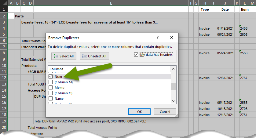
• This brings up the Remove Duplicates pop-up. Select or unselect columns as desired so that the data being searched is only those columns you want. As an example, in a customer list, you probably would not want to remove duplicates from the zip code or city columns.
• Once the correct columns have been selected, click the "OK" button.

A pop-up will show how many duplicates were found and removed in addition to how many unique values remained.

Excel is a very powerful spreadsheet tool that can easily handle and process large amounts of data. Unfortunately, over time, a workbook can feel somewhat bulky and inefficient. Knowing how to use some of the built-in, but often unknown, features is key in continuing to use Excel in an efficient manner. Some of these features include being able to go directly to any tab, hiding columns or sheets, in addition to extending the number of viewable tabs.

As always, software applications often have features we are unaware of, but those tricks can make all the difference in its usability.