Organizational Tips

Using Conditional Formatting to Identify Date-Based Patterns in Excel

Wendy Howell

Sep 9, 2022 • 4 min read

There are lots of ways to use Excel to track data patterns. Using conditional formatting is a way to automate pattern identification and can be especially helpful when working with larger sets of data. In our previous post on conditional formatting, we discussed items like how to color code top, bottom and average values, how to color numbers on a sliding scale, how to use icon sets and more.

This post continues this topic by showing how to use conditional formatting to identify date-based patterns in Excel.

A video showing how to add conditional formatting to identify date-based patterns.

Using Conditional Formatting to Identify Date-Based Patterns in Excel

Adding date-based conditional formatting in Excel is an easy way to help identify important upcoming dates, dates that have passed, and much more.

To set up conditional formatting to identify patterns based on date:

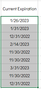
Open a spreadsheet that has a column with dates tracking something like renewal period, last contact, or anything that makes sense for you.
Select the cells with dates in them, or select the entire column or row where you want to apply the conditional formatting.

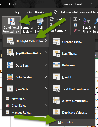
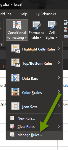
Select the date fields or select the entire column/row to apply conditional formatting to.

Click on "Conditional Formatting" on the Home tab.
Click on "Highlight Cells Rules" to expand the menu.
Click "More rules" at the bottom of the pop-out window. This will open the new formatting rule dialog box.

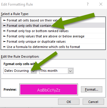
Open the menu for conditional formatting and select more rules in the "Highlight Cells Rules" menu.

Click on "Format only cells that contain" as the rule type.
Select "Dates Occurring" from the drop-down menu under the heading "Format only cells with:".
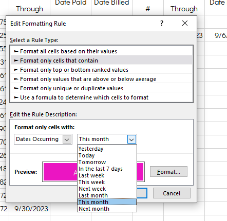
Set the date you want highlighted by this rule. The date choices are: yesterday, today, tomorrow, in the last 7 days, last week, this week, next week, last month, this month, and next month.
Click the "Format..." button next to Preview at the bottom and set how the content will be formatted when it meets the criteria you have set.

Use the "Format only cells that contain" rule type to use dates as the conditional formatting criteria.

There are several date choices to choose from.

Click "OK" once the rule is set the way you want. This will bring you to a window showing the current rules.
Continue adding rules until you have all the rules you want.

NOTE: To view the current rules, or edit a rule later, click on "Conditional Formatting" and select "Manage Rules" from the bottom of the drop-down list.

To edit a rule or view the current rules, simply go to "Manage Rules".

Adding rules with custom dates

Although there are many different types of dates you can select from, being both in the future and in the past, this list is by no means exhaustive and there are times when it does not meet your unique needs. Luckily, there is also a way to set custom dates with conditional formatting highlight rules.

To create conditional formatting rules with custom dates:

Select the cells to apply the formatting to and open "Highlight Cells Rules" from the conditional formatting menu.
Choose "More rules" from the bottom of the list.
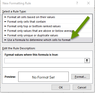
In the New Formatting Rule box, select "Use a formula to determine which cells to format" as the rule type.

Choose "Use a formula to determine which cells to format" to set custom date-based formatting.

Enter the formula for the dates you want to highlight in the following format: "=TODAY()-A1>X" where A1 is the cell number of the first cell with a date you want to check against, and X is the number of days after today that you want today compared to.
Set the formatting of the cells for those dates that meet the criteria of the custom rule.
Click "OK" when finished customizing the rule.

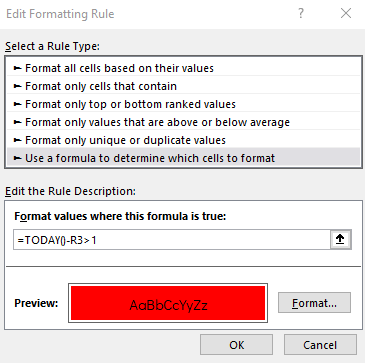
Type a formula for the unique formatting you want to apply to your dates.

In this example, you might wonder why you would want to create a custom formula when selecting "Dates Occurring" to "Yesterday" would seem to provide the same results as the formula above. However, the formula above is quite different as it will highlight any cell with dates that are in the past, regardless of how long ago. So in my example, any date that has passed by a single day, or 100+ days, will be highlighted in red because of the custom date-based conditional formatting rule.

If you were tracking communication, you might create a formula more like this: "=TODAY()-A1>60" which would highlight cells with dates around two months old.

You can also create custom formulas for future dates using the same format, but with negative numbers. The negative number tells Excel that the date has not yet happened. A formula to look for items happening six months from now would look like: "=TODAY()-A1>-180". Again, A1 is the first cell where dates exist to compare to and -180 is the number of days in the future you want to compare against. Each of these can be customized to your unique needs.

Conditional formatting is an extremely powerful attribute available in Excel. One of the best uses for conditional formatting is to track important data, which can include dates. Time and dates can sometimes be tricky to work with in mathematical computations. Luckily, Excel makes it easy to implement conditional formatting based on preconfigured date ranges as well as custom date formulas.

As always, knowing how to create formulas and set up conditional formatting saves tons of times sorting through data looking for patterns later!

Using Conditional Formatting to Identify Date-Based Patterns in Excel

Sign up for more like this.