How you Can Access Rows or Columns in Excel that Fail to Unhide
Excel is a great tool for tracking items, adding conditional formatting to data, looking for trends in data, having complex formulas auto-calculate, managing data choices based on previous selections, and so much more. Every time you think you know quite a bit about Excel, someone else will come along and show you something you never knew. Excel is consistently like that, and if you stick with it, you can accomplish so much with it and save yourself lots of time. Unfortunately, there are times when it can also be frustrating.
This post discusses how you can access rows or columns in Excel that fail to unhide when you select this from the popup menu available for all rows and columns.
How you Can Access Rows or Columns in Excel that Fail to Unhide
Hiding rows or columns in Excel can be useful for many reasons, including, but not limited to:
- Hiding data you do not want to delete, but are not necessary and make it easier to see relevant data to perform certain tasks.
- Removing data from the viewable screen to highlight certain data easier when working with others.
- Removing data from the viewable screen to prevent the data from accidentally being overwritten.
- Hiding data you are not sure you need to keep, but are not ready to delete.
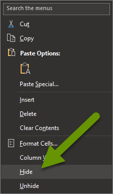
Hiding rows or columns can be done quickly, simply right click on a row or column and selecting "Hide" from the pop-out menu. Keep in mind, you can also select several rows or columns at a time and hide them all at once.

When a row or column is hidden, there are a couple of ways you can tell:
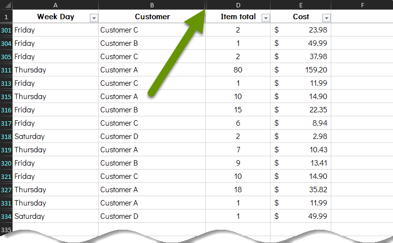
- The labels for the rows or columns skip a value. For example, in the image below, you see the columns skip from column B to column D.
- The lines where the row or column would be still exist, but they are really close together.

If you are working in a really large spreadsheet, it can be very easy to scroll right past a hidden row or column and not notice the missing value. It is even easier to miss the lines that are really close together representing those hidden rows or columns. However, once you see them, if you select the rows or columns surrounding the hidden row or column, you can right-click and select "Unhide" from the pop-out menu to expand those columns and view the data in them.
Unfortunately, sometimes you can try unhiding columns and they do not appear. You can click directly on the row or column or grab the rows and columns around the hidden row or column and select unhide, but nothing happens.
The reason the rows or columns are not viewable is not due to being hidden. The rows or columns are not viewable because they have been resized to take up the smallest amount of space, which happens to match the size they would be if they were truly hidden.
In this situation, the row or column is not viewable, the heading value cannot be seen, and there is a small line where the row or column should be. Since the way this looks points to the fact that the row or column is hidden, it can be frustrating when you try to unhide the data and nothing happens. Luckily, there is a way to fix this issue.

When a row or column is resized, right-clicking on the row or column and selecting to "Unhide" it will not work. Instead, you need to resize the column or row by dragging its size down or to the right enough so that the data can be visible. While this is not difficult, it is important to realize that there are several reasons why the data is not viewable, and what you can do to get access to the data.
Using hidden rows and columns in Excel is a really convenient tool when you are working with larger sets of data or need to focus only on certain aspects of the data included in the spreadsheet. However, resized rows and columns can look exactly like hidden rows and columns so if you try to unhide data and nothing happens, try resizing those rows or columns to get access to the data.
As always, knowing additional ways to accomplish the same task come in handy!

