How to Create Forms in Excel With Cascading Lists that Control Data Input

Excel is a very powerful application, and as such, we have discussed several topics about what it can do including how you can use it to save time, organize data, find patterns, find data outliers, manage data input using predefined lists, chart data over time, and much more. In this post we will build upon a previous post where we discussed how to create predefined lists to control the data inputted into a field.

This post will demonstrate how to create cascading lists where list options are dependent upon previous list selections in Excel.

How to Create Forms in Excel With Cascading Lists that Control Data Input

If you are not familiar with, or cannot recall, please first read our original post how to control the data inputted into a field in Excel.

One of the greatest benefits of using drop-down lists in Excel fields is that you can control the data that is entered into the field, effectively preventing bad data entries. Additionally, lists save the person entering the information time!

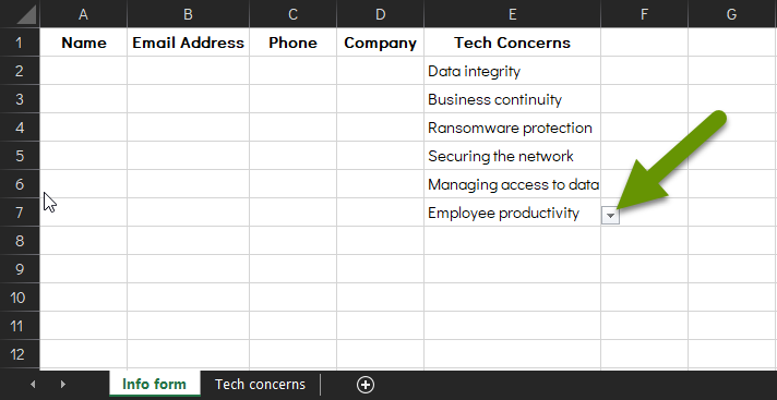
In this post we will use the example of a form created to collect data from potential or existing clients about the types of concerns they have with their technology. If we were to list all of the items a company or person might be concerned about, the list would be overwhelming and we likely would not get great results.

Consider walking into a store of any type looking for a single item of which there are 50 variations. In all likelihood you will do one of two things:

• Go straight to the one version you already know you like and purchase it.
• Browse through a bunch of different options until you feel exhausted by the choices and walk away without making a purchase.

Obviously there are options in between, but they are less likely to occur. In the case of gathering information, such as a form, if you narrow down the choices a user must make, you can increase their engagement and get better feedback.

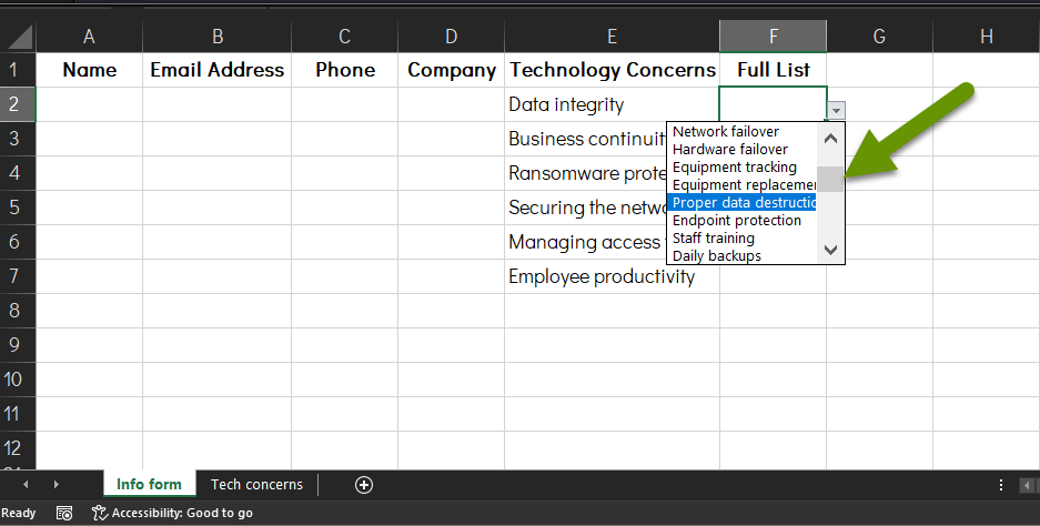
In this example, we are going to create a form with a drop-down list in one column showing concerns by type, using data validation to control the list. The content for the drop-down list will be located on a separate tab to keep the information isolated from the form data. If we listed all of the topics of concern without using cascading lists, we would have over 30 items.  Instead we will group these into six unique categories that a user can choose from in our drop-down list:

This is a much more manageable approach than having the list look like this where the user would have to scroll within the drop-down list window to see all the options:

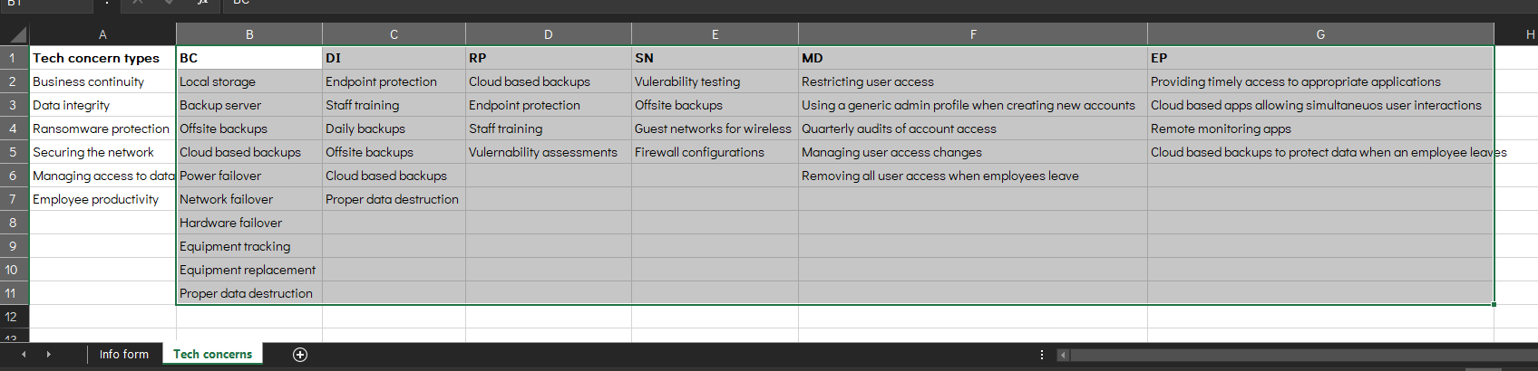
• With the drop-down list of categories created, you next need to list all the options available for each category.

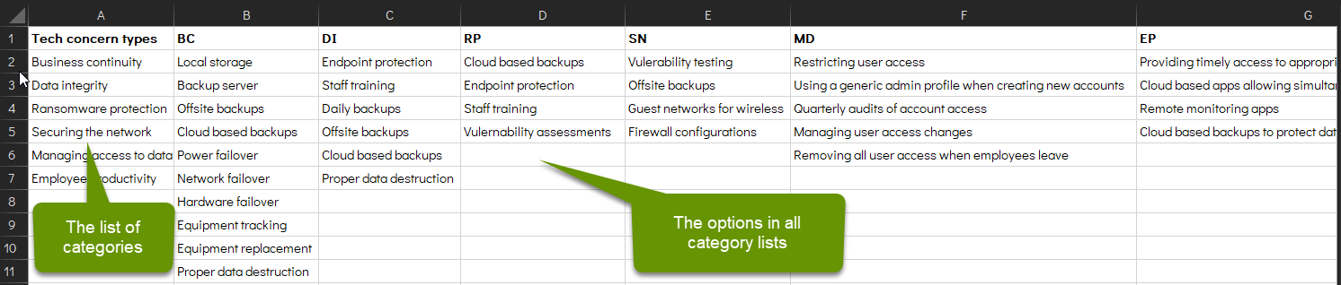
We will link each category in the list to the specific options we want to provide in a cascading list. You may notice that I shortened the titles of the category titles above their lists because we will be typing these in our data validation box and the more succinct they are, the easier this is to accomplish.

With the categories and their options listed, you will need to create a selection of this data.

• Click on the Formulas tab in Excel.
• Highlight the category headings and their options below - leaving the original category list out of your selection.

• With the data highlighted, click the "Create from Selection" button in the Defined Names section on the Formula tab.

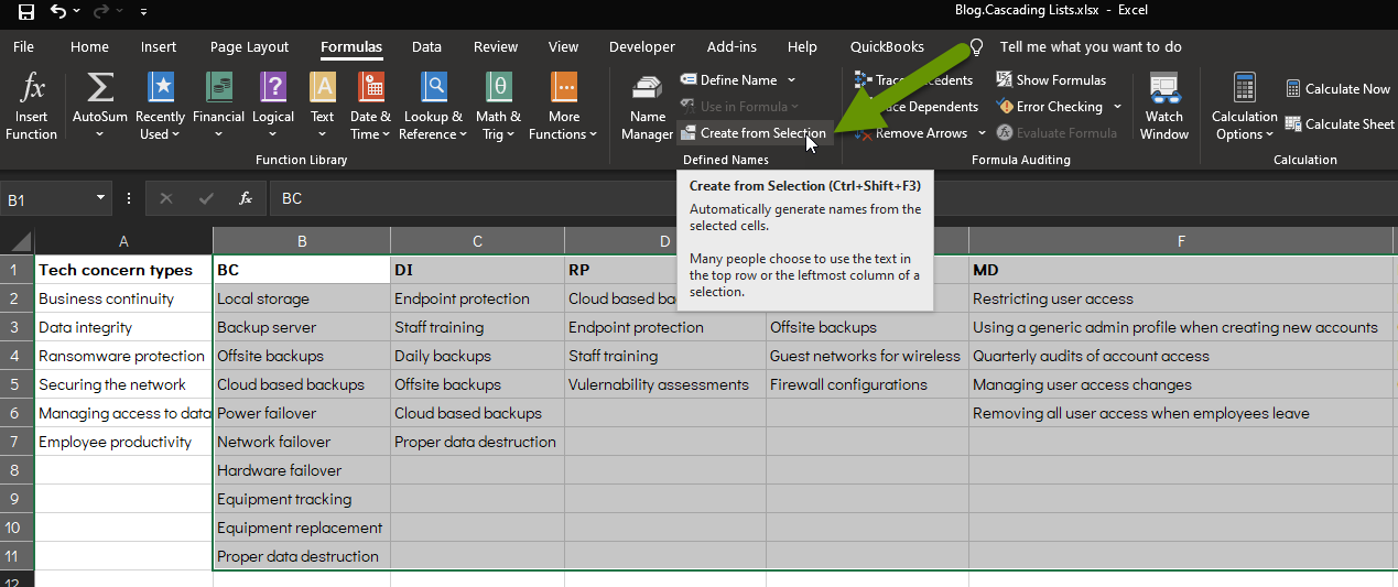
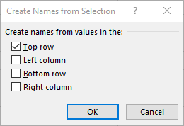
• When prompted for the names for the selection, check only the box next to "Top row" as long as that is where you have your category titles, as we do in our example.
• Click the "OK" button to save the selections.

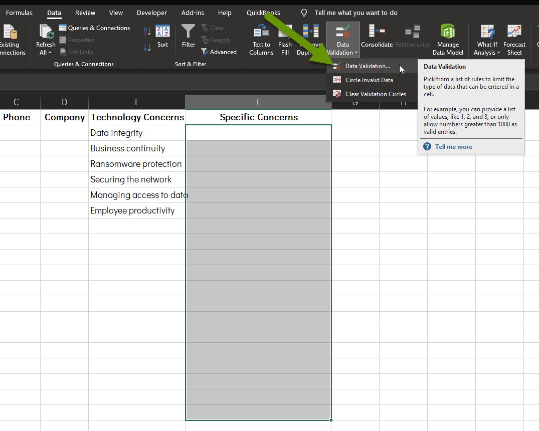
• Back on the tab where the form is, add a new title next to the category list.
• Highlight all of the rows where you want the cascading list options to appear and click on the Data Validation button on the Data tab.

• In the Settings tab of the Data Validation box, select "List" from the drop-down under the "Allow:" heading.

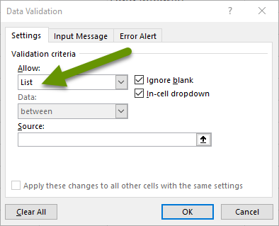
• Click in the "Source:" box.
• Enter a formula using the selection you created in the last step.

NOTE: When working with a formula like this, where the input box is small and can be difficult to move within, I use an application like Notepad so I can see all of the formula at once. This makes it easier to troubleshoot if you run into issues and you can copy and paste it into the Source: box to test.

In our example, our formula looks like this:

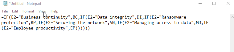
The formula needs to be formatted like this:

• Begin with "=IF" to start the statement.
• Follow up with "(cell number to check to see which category was selected=
• Next enter the category name with full quotes around it, "example category". NOTE: These are case sensitive, so be sure they match exactly.
• Follow this with a comma, then enter the heading above the category options that matches the category you listed. These can be the same, or they can differ. Follow with a comma, and begin the next IF statement.
• From here the formula repeats for all categories until none are left.
• Be sure you end with as many closing parenthesis as you have opening parenthesis.

NOTE: If you run into errors when you try to save the formula, double check all of the formula formatting. Be sure the commas are only where they should be. Verify the names match the headings you have selected. Double check to see if the selections were created correctly by going to the formula tab and clicking "Name Manager" which will give you a list. Lastly, make sure the format of the cells is set to General or Text.

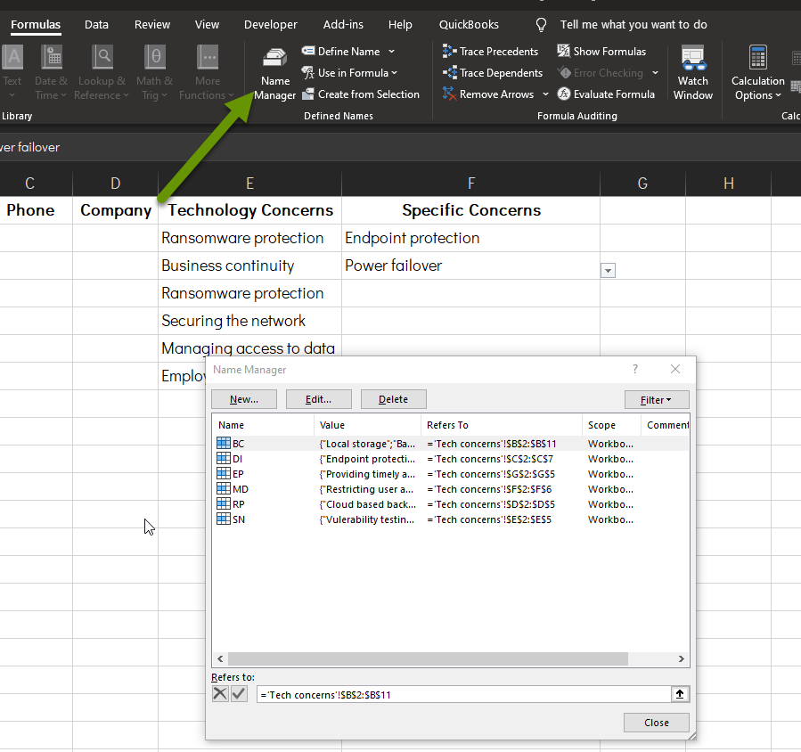
Bonus note: You can modify the cells included when you originally created the named selections in the Name Manager if not all of your lists were the same length. Simply click on the name of the appropriate category and update the cells in the "Refers to:" section, then click the green check to save.

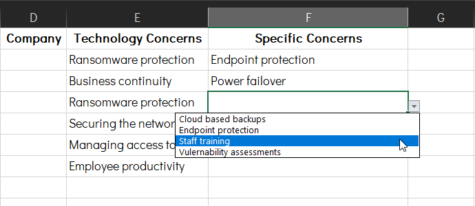
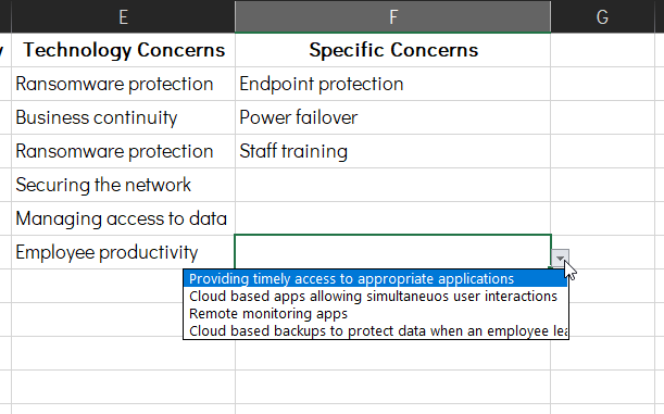
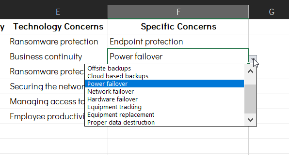
Once you have correctly entered the formula, the second drop down, or cascading list, will show only those options in the secondary column based on the category list chosen in the first.

Here are a few images of this in action using our example:

Having cascading lists, or lists whose options are based on previous choices, in Excel forms is a great way to control the data being inputted while also gathering more consistent and precise data from the person filling out the form. Luckily, setting up categories and creating list options for each category can be done fairly quickly.

As always, knowing what applications are capable of helps us choose how best to utilize them effectively!