How to Control Data Entered into Cells using Drop-Down Lists in Excel

Excel spreadsheets can be a great way to collect information. However, how valuable that data is depends greatly upon the conformity of the data inputted. One way to keep the data uniform is to control the data that is entered by inserting drop-down lists with preset selections that users can choose from. This is especially helpful when multiple people are entering data.

This post discusses how to control the data that can be entered into certain columns by adding drop-down lists with preset options.

The following video demonstrates how to accomplish this:

How to Control Data Entered into Cells using Drop-Down Lists in Excel

Inserting a drop-down selection into a column or set of cells forces users to choose from the preset list, allowing the creator of the spreadsheet to control the data a user can enter. This can prevent users entering incorrect data, or data in a format that is unusable to the creator of the spreadsheet. Some quick examples of where preset data can be helpful are:

• Listing states in a 2-digit format - prevents full state names, misspellings, and slang like "Cali".
• Having yes or no answers be "Y" or "N" - prevents variations like yes, yeah, yah, nah, nope, etc.
• Using "New" or "Returning" for customer type - prevents different versions of the same word like recurring, previous, repeating, etc.
• Zip codes - to prevent typos when you are collecting from a smaller demographic where the zip codes can all be accounted for.
• Any other question where you have a specific set of answers you want users to choose from.

The examples above show several variations of answers users might enter if asked to fill in an answer. Obviously there are others which proves how important it can be to control data for consistency so you can use the data more effectively.

Creating drop-down selection lists in Excel

Before creating a drop-down selection list in Excel, first decide which column(s) you want to add selections to as well as what the selection options will be. Planning this ahead of time will significantly reduce the amount of time it takes to create the drop-down lists.

• Open a new or existing spreadsheet in Excel.
• (Optional) If the spreadsheet is new, create headings for the columns.
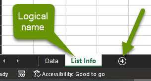
• Click to add a new sheet that will be used to define the preset data used in the drop-down lists and name the sheet something that makes sense. NOTE: Storing the list options in another tab helps protect the data set up for these lists.

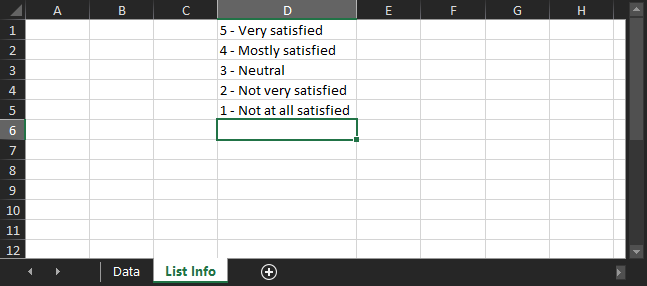
• In the newly created sheet, enter all the answers you want to appear as options in the drop-down list for a column or group of cells in another sheet. NOTE: Be sure to enter the answers in the order you want them to appear in the list.
• For this example, we are tracking customer satisfaction with the order process.

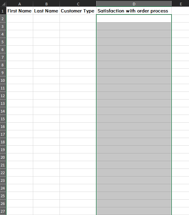
• Highlight the cells where you want to insert the drop-down list.

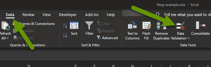
• Click on the Data tab and click on "Data Validation".

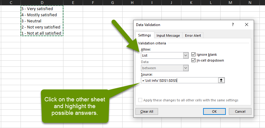
• In the Data Validation box, select "List" under the Allow: heading on the Settings tab.
• Click in the Source box to select the preset answers. Click on the spreadsheet tab where you listed the answers and highlight all of them.
• Click "OK" in the Data Validation box to save these settings.

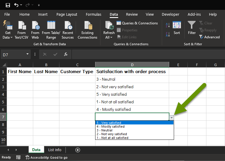
If you toggle back to the main sheet, you can now select the options you set from the drop-down list that appears next to each cell.

• Continue this process to add all of the necessary preset drop-down lists.
• Verify each drop-down list in the other sheet works as expected.

(Optional) Hide the sheet with the list of options

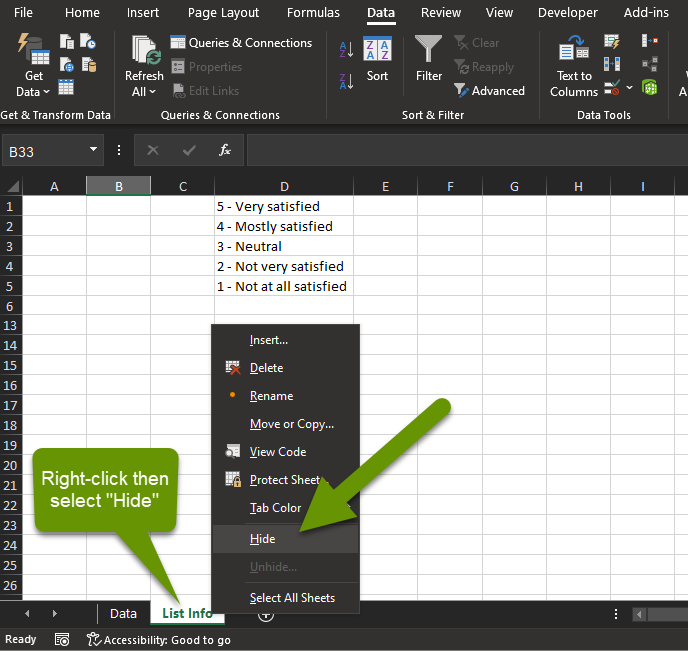
If desired, you can hide the sheet where you created the preset list answers. This can help prevent users from accidentally modifying the data in each list. To hide the sheet:

• Right-click on the title of the sheet at the bottom of Excel and select "Hide" from the pop-up menu.

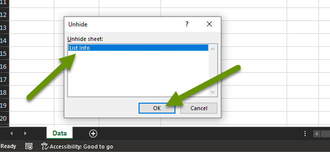
If you ever need to update the answers in a list, remove a list, or add a list, you can do this easily by unhiding the sheet with the list answers. To unhide a sheet:

• Right-click on the name of an existing tab.
• Select "Unhide" from the pop-up menu.

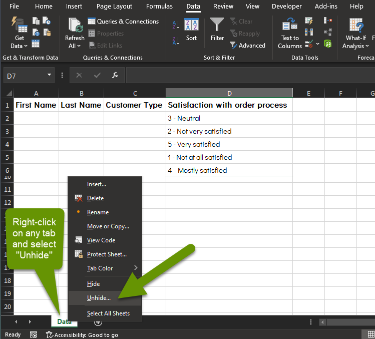
• Click on the name of the sheet to unhide and click "OK".
• The sheet will automatically be visible again.

Creating drop-down lists allows you to control what answers users can enter in certain columns. This helps provide better data because it controls the formatting of the data, which can make it much easier to filter through and analyze. Additionally, the sheets with the preset answers to the drop-down lists can be hidden so users do not accidentally modify this data. If needed later, these sheets can be unhidden so the data can be updated, added to, or removed.

As always, knowing how to manage the format of data ensures the data is uniform, and therefore, more valuable.