
3 Ways to Increase Excel's Usability and Ease of Use

Microsoft's Excel is one of those programs that once you begin using it, you realize the genius of it and continually find new uses for it. However, Excel has a slightly bigger learning curve than an application like Word. Anyone opening Word can quickly imagine typing a document of some sort whereas practical uses for Excel are often more illusive, that is until you become more familiar with it.
This post discusses three ways any user can increase the usability and ease of use of Excel. Also, the following video covers the same information:
3 Ways to Increase Excel's Usability and Ease of Use
This post discusses the following ways to increase the usability of Excel:
- Resizing columns and rows to auto-fit the content
- Resizing columns or rows when content is wider than the window
- Using the hide column/row feature to share information without giving users access to all data
Resizing columns and rows to auto-fit the content
One thing that can be annoying about Excel happens when entering information. Over time, when data is too big for a cell it is cut off or will spill over if the cell next to it happens to be empty. The data is not actually in the second cell, it just spans across visibly until information is entered into that cell which will cut it off.
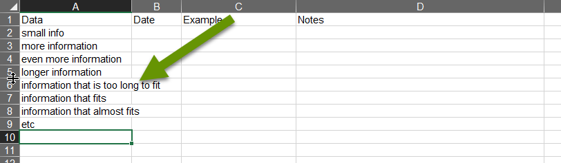
This is a common experience because as a worksheet is being set up, the columns and rows are initially set to a predicted width. As data is entered, this set size often turns out to be too narrow. Resizing a column or row once the content overlaps is easy, but might need to be done several times while entering data into a worksheet. If you are manually adjusting the content, it requires scrolling to find the cell with the most content which is a waste of effort.
Luckily, there is a better way to handle the data in a column or row - using the auto-fit feature. This automatically resizes the column or row to just bigger than the cell with the largest amount of content.
To resize columns or rows to autofit for all the content in a column or row:
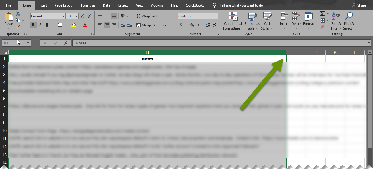
- Move the mouse between two columns or rows in the header section. The header section is represented by letters for columns and numbers for rows. Place the mouse to the right side of the column or below the row you want to auto-size.
- When you have the icon with a thick solid vertical line and a double-arrowed horizontal line, double-click to auto resize the column width or row heigth.
NOTE: If you ever need to reduce the size of the column or row, click in the same header location and drag horizontally for columns or vertically for rows to the desired size.
Resizing columns or rows when content is wider than the window
Sometimes a column or row can have so much data in it that once resized, it is wider or taller than the Excel window. Trying to resize this back down can be problematic. Using the scroll buttons at the bottom of the worksheet jump past the column or row making it impossible to grab between the headers to resize them. Luckily there is still a way to resize these oversized columns and rows.
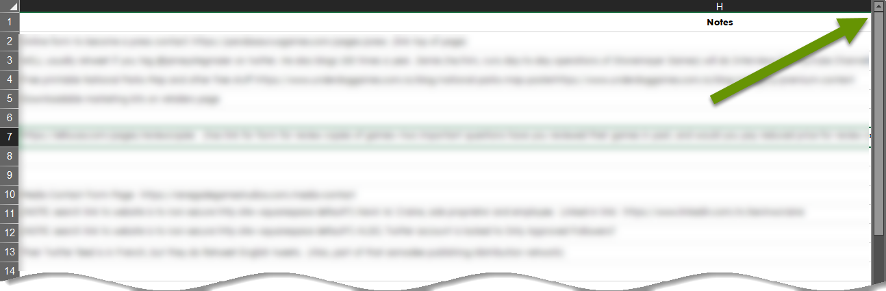
To resize columns or rows after they have expanded beyond the viewable window due to the amount of content:
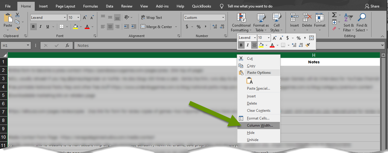
- Right-click in the header section of the column or row that needs to be resized. The header section is represented by letters for columns and numbers for rows.
- Select "Column/Row Width" from the drop-down list.
- Change the size of the column width to something much smaller so it falls within the viewable window. From there, you can manually slide the header for that column or row to a size you like.
- Click the "OK" button and the column or row will resize.
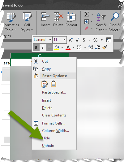
- Click on the header above or to the left of any column or row and right-click the mouse.
- Select "Hide" from the pop-up menu.
- This will hide the column or row - showing only a small space between two column or row border lines in the header row.
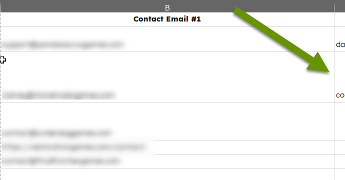
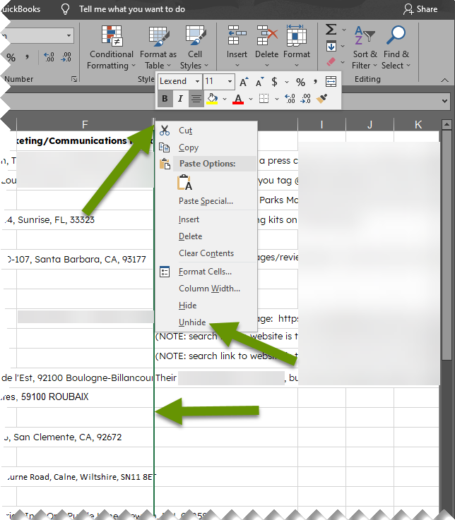
- Move the cursor over the top of the small two-line gap in the header where the column or row is hidden. (See image above)
- With the icon in the shape of a thick solid vertical light and a double-arrowed horizontal line, right-click and select "Unhide".
- NOTE: If you are in the correct location, a very thin line representing the hidden column or row will be highlighted. If instead, one of the columns or rows next to the hidden column is highlighted, you have not correctly selected the hidden column or row.
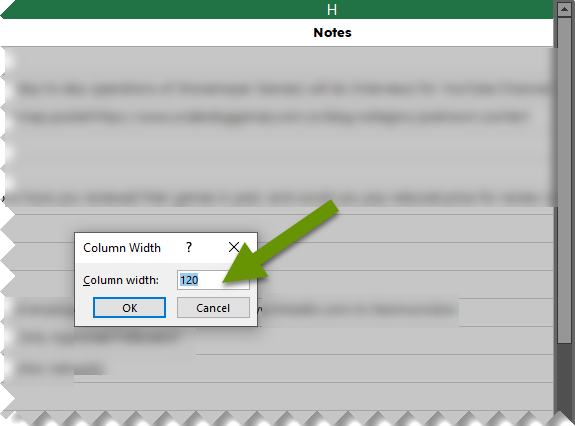
With the sizing changed, the column or row should fit back inside the window. In the example below we dropped the size from 255 to 120 and as you can see, the column once again fits within the viewable window.
Using the hide column/row feature to share information without giving users access to all data
There are lots of reasons why you might want to hide a column or row. First, hiding information in a column or row is an amazing feature because it keeps it from being presented without removing any data! You may want to hide data because it has information about people that is sensitive or identifies them, or because it is financially sensitive, or maybe it is as simple as taking up valuable real estate in a situation where that particular information is not needed.
To hide a column or row:

To unhide a column or row:
One last thing to note, if you hide data in an Excel worksheet and share that file with others, they can unhide the data at any time. This means you will not want to hide sensitive data thinking you are protecting it.
There is still a way to share information without giving access to hidden data. First, hide the column(s) or row(s) with the data you prefer not to share. Then save the worksheet as a .pdf file where the hidden columns cannot be revealed.
Excel worksheets can be extremely powerful, but like any powerful application, there can be a steeper learning curve. This post discusses three things that can increase the usability and ease of use of Excel so users can become more familiar with it and its many uses. Resizing columns and rows for best fit and to fit on the viewable screen, as well as hiding unnecessary data are a few tips that most users can benefit from.
As always, knowing how to modify an application to best meet your needs makes it more efficient and usable!